stisblazefix Documentation
Warning
Please note that AURA/STScI is not responsible for any damages resulting from the use of this software.
The stisblazefix python module is designed to empirically correct STIS echelle data
for misalignment in the blaze function. It does this by shifting the overall sensitivity
curve applied to each order to find the shifts that make the measured flux in the
wavelength overlap of adjacent echelle orders most consistent, under the assumption that
the shift to be applied to each echelle order is a linear function of the order number.
Once installed, the fluxfix function of the module can be run by supplying a list of
STIS echelle x1d FITS file names, as well as an output name to be used for the PDF
diagnostic plots produced. For example:
stisblazefix.fluxfix(['ocb6i2020_x1d.fits', 'ocb6f2010_x1d.fits'], 'example.pdf')
This will produce as output the files ocb6i2020_x1f.fits and ocb6f2010_x1f.fits with
corrected values for the extracted flux and error vectors, as well as a PDF file with a
diagnostic plot for each exposure showing changes made to the data.
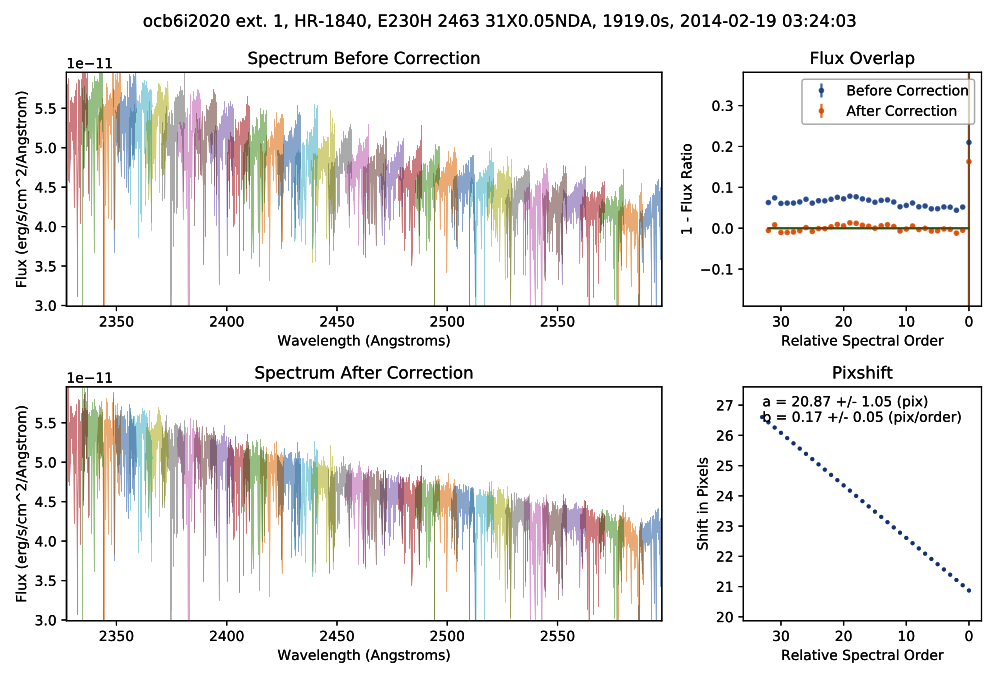
Example blaze correction to HST/STIS E230H dataset OCB6I2020.
See also
See STIS ISR 2018-01 for details on the correction.
Installation
The stisblazefix package has been updated to install via pip:
pip install stisblazefix
Dependencies
It requires numpy, scipy, astropy, matplotlib, lmfit.
Warning
Requires at least numpy 1.13; bugs occur with numpy 1.12.
Manual Installation
Alternatively, you may download and manually install stisblazefix via:
pip install .
Python API
Most users will be interested in the fluxfix function.
- This module contains the following functions:
findshift: calculates the shift to the blaze function that best aligns the spectrum.fluxcorrect: takes a shift to the blaze function and recalculates the flux and error.fluxfix: takes a list of x1d fits files and generates corrected x1f files and diagnostic plots.generateplot: takes an old and corrected spectrum and generates a diagnostic plot.plotblaze: plots the sensitivity curves for an extracted spectrum.residfunc: wrapper for lmfit minimizer.residcalc: calculates the flux residuals for the overlapping regions of an echelle spectrum.
- stisblazefix.findshift(filedata, guess, iterate=True)
Find pixshift that best aligns spectral orders.
Use lmfit to calculate the pixshift (to apply to the blaze function) as a linear function of relative spectral order that minimizes the flux overlap residuals as calculated in residcalc.
filedata: the data attribute of an x1d FITS file.guess: a tuple containing the starting parameters for the fit.iterate: Boolean that determines whether the function iterates to find the best fit.
Returns pixshift, the error in the pixshift, and the final parameters.
- stisblazefix.fluxcorrect(filedata, pixshift)
Recalculate and return corrected flux and error vectors, based on shifted blaze function.
filedatais the data attribute of an x1d fits file.pixshiftis a 1D vector with length equal to the number of orders in the echelle spectrum. It contains the shift of the blaze function in pixels as a function of relative spectral order.
- stisblazefix.fluxfix(files, pdfname, guess=None, iterate=True, nxplot=1, **kwargs)
Corrects STIS echelle spectra by aligning the sensitvity function to compensate for shifts in the blaze function.
This routine will iterate over a list of STIS echelle x1d files and for each exposure in each file it will find the shifts of the sensitivy curves for the spectral orders that maximize the flux consistency in the overlap between orders. Corrected flux and error vectors are then calculated and saved to new output files where _x1d.fits is replaced with _x1f.fits.
It assumes that amount by which the sensitivity curve for each spectral order needs to be shifted is a linear function of the order number. The optimal shifts for each exposure to minimize the flux inconsistency in the overlapping regions of the spectral orders are found. Each exposure is treated independently.
Args:
files(list of str): A list of file names corresponding to STIS echelle x1d files. All file names should end in _x1d.fits and should contain extracted and flux calibrated STIS echelle spectra output from CalSTIS.pdfname(str): Name for the output PDF file.guess(tuple of two floats): Contains a starting guess for the linear relation used to shift the blaze function. Should be in the form (a, b), where the blaze shift for each spectral order x will be a + b*x. Defaults to None, which then substitutes a suitable guess supplied in the code.iterate(bool): When set to True the code will iterate to find the values for a & b that minimimize the inconsistency in the flux ovelap regions. When set to False, the code will use the values supplied in Guess without iterating. Defaults to True.nxplot(integer): default 1. When set to a value > 1 will add extra plot pages, each comparing the original and corrected spectrum over approximately 1/nxplot of the wavelength range, but allowing a slight wavelength overlap between the plots.- Returns:
A list of dictionaries, one for each exposure found in the x1d files. Each list element contains:
pixshift: array of pixel shift values applied to sens curveacof: offset applied to sens curve of lowest orderbcof: change in offset per orderacoferr: formal error in the value for acofbcoferr: formal error in the value for bcofoldresids: vector of residual flux differences in order overlaps of original dataoldresiderr: error vector for oldresidsnewresids: vector of residual flux differences in order overlaps of corrected datanewresiderr: error vector for newresidsfilename: input file nameextno: extension number of input file for this exposure
- Produces:
A new copy of each x1d file with the fluxes and errors corrected for the new shift of the sensitivity vector. The new files replace x1d in the file names with x1f.
A multipage PDF file with diagnostic plots for each exposure.
- stisblazefix.generateplot(origdata, newflux, newerr, pixshift, params, paramerr, oldresids=None, oldresiderr=None, ntrim=5)
Generate a diagnostic plot for a corrected spectrum.
Plot spectrum and residuals before and after correction to blaze function, and pixshift vs relative spectral order. Return a figure object.
origdata: the data attribute of an x1d FITS file. This should contain the original flux.newflux: the corrected flux.newerr: the corrected error.pixshift: a 1D vector with length equal to the number of orders in the echelle spectrum.
- kwargs:
oldresids: the residuals for the uncorrected data.oldresiderr: the error in the residuals for the uncorrected data.ntrim: the cut made to the edges of the orders to avoid various edge problems. Defaults to 5.
If neither
oldresidsoroldresiderris passed, they will be calculated fromorigdata.
- stisblazefix.plotblaze(filename, pdfname, ntrim=7)
Plot the blaze function for each order of a STIS echelle spectrum.
- stisblazefix.residcalc(filedata, flux=None, err=None, dq=None, ntrim=5)
Calculate and return the flux overlap residuals and weighted error.
Flux residuals are calculated by summing the flux in the overlapping region in adjacent orders, taking the ratio, and subtracting from one.
filedatais the data attribute of an x1d FITS file.- kwargs:
flux: flux vector the same size as the flux in filedata.err: error vector the same size as the error in filedata.dq: data quality vector the same size as the dq in filedata.ntrim: cut made to the edges of the orders to avoid various edge problems. Defaults to 5.
If either
fluxorerroris passed, they will be used to calculate the residuals. Otherwise, the flux and error arrays fromfiledatawill be used.
- stisblazefix.residfunc(pars, x, filedata)
Wrapper for lmfit minimizer. Return weighted residuals for a given pixshift.
pars: a tuple containing lmfit parameters.x: the input variable, in this case relative spectral order.filedata: the data attribute of an x1d FITS file.
Simulations of Blaze Shift vs SNR
We performed simulations on the performance of stisblazefix for a range of signal-to-noise (SNR) levels as part of the ULLYSES DR7 reduction in order to determine the behavior of the algorithm at lower SNR, and thus when to apply it. We used observations of STIS standard white dwarfs from the MAMA Spectroscopic Sensitivity and Focus Monitor programs.
We estimated the average continuum SNR of each echelle X1D dataset by taking the FLUX/ERROR column ratio, trimming out 100 pixels from both edges of each order, calculating the 75th percentile value for each order, and taking the mean across all orders. This proved to be robust to emission & absorption lines and to the blaze function edge behavior.
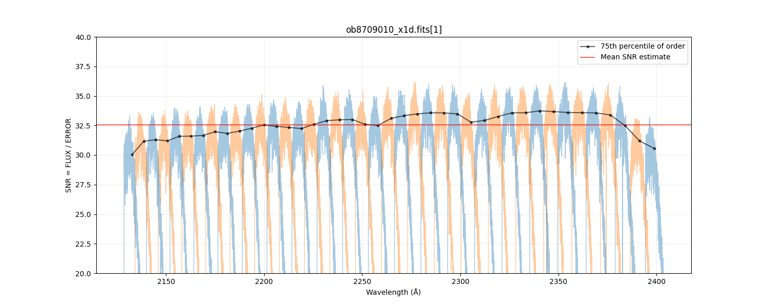
An estimate of the continuum SNR for an example E230H/c2263/0.2X0.2 dataset.
We randomly subsampled the measured counts in the monitor datasets at levels of [0.5, 1, 2, 5, 10, 25, 50]%, giving a range of continuum flux levels, and corresponding SNR. The subsampled datasets were processed with CalSTIS and stisblazefix to derive the blaze shift offset at the far orders and the mean across all orders. We differenced these values with those derived from the corresponding full dataset.
When plotted against SNR, the scatter in the stisblazefix mean blaze correction
increases to >2 pixels at SNR=5 for the M-modes and ~3 pixel at SNR=10 for H-modes. These
thresholds also conservatively correspond to a sudden increase in scatter of the
CalSTIS-calculated blaze shift value (Δ in the SCI ext BLZSHIFT keyword).
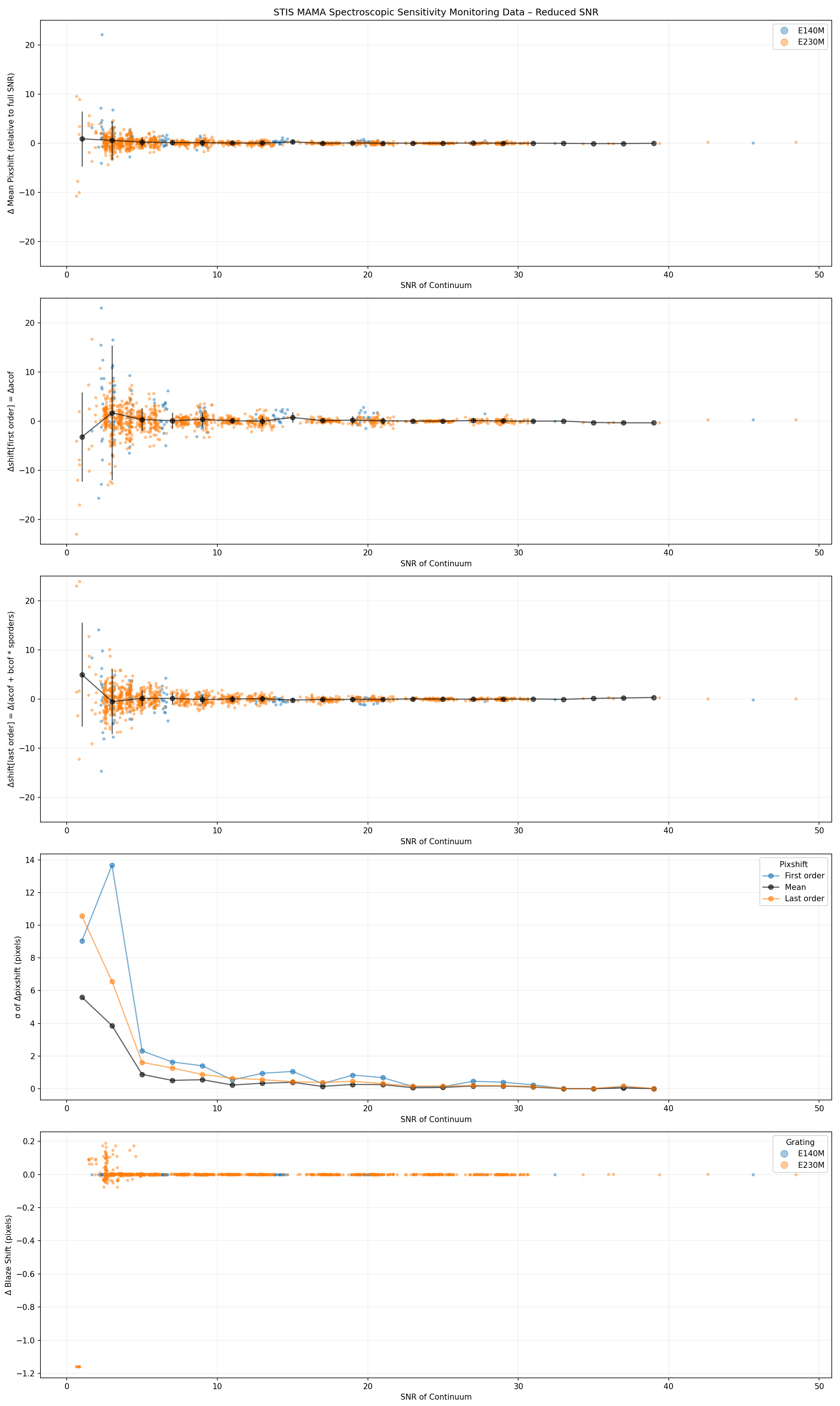
M-modes
Top three panels: The scatter in the stisblazefix empirically-derived blaze shift offset in subsampled monitor data, relative to the full datasets. The panels correspond to the mean, first, and last order of each dataset, respectively. The black points bin the results every 4 SNR.
Fourth panel: The scatter within each SNR bin, showing roughly where the correction becomes unreliable.
Fifth panel: The ΔBLZSHIFT, as calculated by calstis.
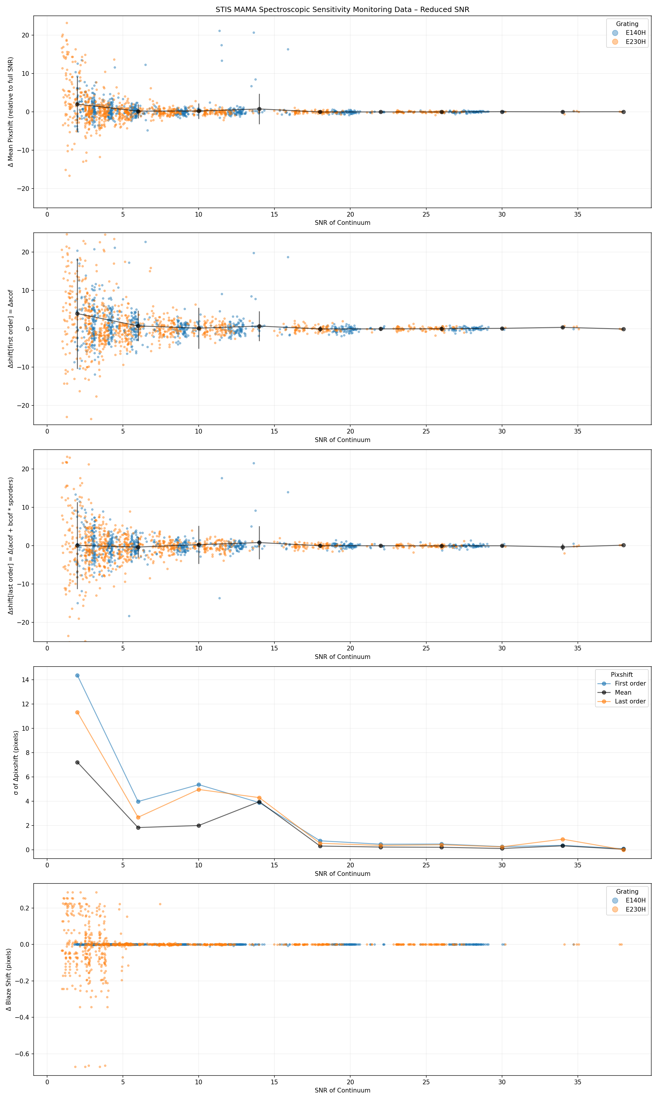
Same as previous figure, except for H-modes.
Release History
v1.0a1: Initial pre-release of stisblazefix package. Additional updates are pending.
v1.0a2: Improved handling of divide-by-zero warnings. Reduced conda package size.
v1.1: Fixed bug in lmfit dependency call when iterate=False.
v1.2: Updated packaging with pyproject.toml and pip installation.
Support
For support, please contact the STScI help desk at https://hsthelp.stsci.edu